import numpy as np
import arviz
import x3cflux
import hopsy
import pandas as pd
import matplotlib.pyplot as plt

Quickstart: the Spiralus Model

This notebook explains the high-level workflow for performing parameter estimation with 13CFLUX. It assumes a model file is already available that defines the network structure, atom transitions, and isotope-labeling experimental details (for example, extracellular rates). For model-specification details, see the libFluxML documentation, the FluxML paper, or the Data Objects section of this documentation.

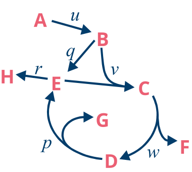
Here we us a simple toy model called the Spiralus from the Primer to 13C Metabolic Flux Analysis.

The input A has two carbon atoms which, of which the first position is \(^{13}\)C labeled, and we have a measurement of the uptake rate u as well as an MS measurement of H. You can download the model from this location.

Building a simulator

We start by building a simulator object, which is the central piece of 13CFLUX. If you know the name of the configuration, you can directly create the object. Exper users may want to specify the argument sim_method, which describes the type of simulation variables used (cumomer, emu). By entering the default auto, the method with less initial unknowns is chosen.

simulator = x3cflux.create_simulator_from_fml("spiralus.fml", "ms_STAT", sim_method="auto")

Alternatively, if the name of the configuration is not known we can print a list, and select the one we would like to choose

data = x3cflux.FluxMLParser().parse("spiralus.fml")
print([config.name for config in data.configurations])

['ms_INST', 'ms_STAT']

select configuration and create the simulator object

config = data.configurations[1]
simulator = x3cflux.create_simulator_from_data(data.network_data, config, sim_method="auto")

The simulator object automatically computes free/dependent parameters, reduces the labeling states by backtracing and pre-computes template labeling systems. Free parameters can be accessed by simulator.parameter_space.free_parameter_names. The order of free parameters is alway netto fluxes, exchange fluxes and pool sizes (for isotopically non-stationary only).

print(simulator.parameter_space.free_parameter_names)

['p.n', 'u.n']

FluxMLData objects can be used to store one parameter configuration (e.g. a suitable starting point for numerical computation). It can be retrieved from the parameter entries of a measurement configuration.

params = x3cflux.get_parameters(simulator.parameter_space, simulator.configurations[0].parameter_entries)
print(params)

[0.4 1. ]

Accessing parameter inequality constraints

Linear inequality constraints \(\mathbf{A} \cdot \mathbf{\theta} \leq \mathbf{b}\) can are accessible through the parameter space object.

ineq_sys = simulator.parameter_space.inequality_system
print(ineq_sys.matrix)
print(ineq_sys.bound)

[[-1.  0.]
 [ 0. -1.]
 [ 0.  1.]
 [ 1. -1.]
 [ 1. -1.]
 [-1.  1.]
 [ 1. -1.]]
[0. 0. 5. 0. 0. 5. 0.]

Forward simulation

Residuals to observed data can be evaluated via the compute_loss function. The simulator object also provides functions to compute the gradients (e.g. compute_loss_gradient) Jacobians and the approximate Hessian matrix (see documentation).

for p in [params, [0.5, 1], [0.8, 1], [0.6, 2]]:
    loss = simulator.compute_loss(p)
    gradient = simulator.compute_loss_gradient(p)
    print(f"at {p} loss : {loss:4.2e}  gradient {gradient}")

at [0.4 1. ] loss : 1.31e-28  gradient [-1.33226763e-12  5.32907052e-13]
at [0.5, 1] loss : 1.62e+02  gradient [ 3600. -1800.]
at [0.8, 1] loss : 4.61e+03  gradient [ 30720. -24576.]
at [0.6, 2] loss : 4.98e+02  gradient [-840. 1052.]

simulated measurements and their Jacobian can be calculated using compute_measurements and compute_jacobian

print(f"simulated measurements at {params}: {simulator.compute_measurements(params)}")
print(f"Jacobian:\n {simulator.compute_jacobian(params)}")

simulated measurements at [0.4 1. ]: ([array([-0.  ,  0.84,  0.16])], [1.0])
Jacobian:
 [[-0.   -0.  ]
 [-0.8   0.32]
 [ 0.8  -0.32]
 [ 0.    1.  ]]

The order of measurements is always Labeling measurements, flux measurements and pool size measurements. Here we compar the simulated measurements to the ones reported in the configuration.

def compare_meas(simulator, ps):
    names = simulator.measurement_names[0]
    real_meas = simulator.measurement_data[0]
    real_meas_stddev = simulator.measurement_standard_deviations[0]
    sim_meas = simulator.compute_measurements(ps)[0]
    width = 0.35      # width of the bars

    for m in range(len(names)):
        n = len(real_meas[m])
        x = np.arange(n)  # the label locations

        fig, ax = plt.subplots(figsize=(8, 4))
        ax.bar(x - width/2, real_meas[m], width, label='Real', yerr=real_meas_stddev[m], capsize=5, color='tab:blue')
        ax.bar(x + width/2, sim_meas[m], width, label='Sim', color='tab:orange')

        ax.set_xlabel('Mass shift')
        ax.set_ylabel('Fractonal labeling enrichment')
        ax.set_title(f'{names[m]}')
        ax.set_xticks(x)
        plt.ylim([0, 1])
        ax.set_xticklabels([f"M+{i}" for i in range(n)])
        ax.legend()
        plt.show()

for p in [[0.5 ,1], params]:
    print(f"Simulated measurements at {p}. Residual {simulator.compute_loss(p):4.2g}")
    compare_meas(simulator, p)

Simulated measurements at [0.5, 1]. Residual 1.6e+02

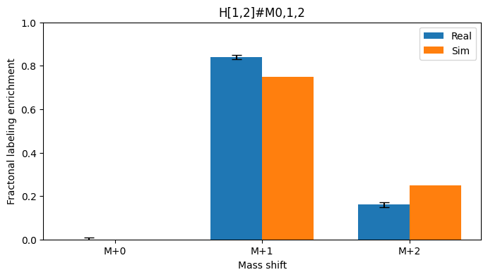
Simulated measurements at [0.4 1. ]. Residual 1.3e-28

Optimization

The simulator object can be directly used for optimization. 13CFLUX provides convenience functions for IPOPT, but is generally compatible with any solver library that support (linear) inequality constraints.

The convenience function must be supplied with the simulator and a starting point. Additionally, custom inequality constraints can be supplied (skipped in this case).Finally, keyword arguments can be supplied to alter the behavior of the IPOPT optimizer (max_iter and tol in our case).

optimum, obj_val = x3cflux.run_optimization(simulator,
                                            starting_point=np.array([0.1, 0.2]),
                                            max_iter=100,
                                            tol=1e-3)
print(f"Found optimum at {optimum} with a loss of {obj_val}")

******************************************************************************
This program contains Ipopt, a library for large-scale nonlinear optimization.
 Ipopt is released as open source code under the Eclipse Public License (EPL).
         For more information visit http://projects.coin-or.org/Ipopt
******************************************************************************

Found optimum at [0.40001103 1.00002669] with a loss of 2.864624265163987e-07

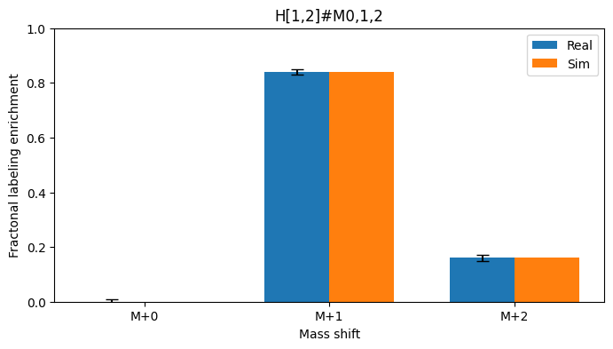
As expected from the low loss, the simulated measurements are very close to the real measurements

compare_meas(simulator, optimum)

Multi-start

For real life problems it is it is recommended to start the optimization from several well dispersed points, to avoid getting stuck in local minima. For this we draw uniform samples from the feasible flux space

samples = x3cflux.run_uniform_sampling(simulator, num_samples=100)

These samples then serve as starting points for the optimization. To make use of parallel compute ressources this can be done in several independent processes (num_procs).

We have a look at the top 5 optima, which all essentially agree

optima, obj_val = x3cflux.run_multi_optimization(simulator, starting_points=samples,
                                                 max_iter=100, tol=1e-3, num_procs=4)
sorted_idx = np.argsort(obj_val)
print("Top 5 optima")
for i in range(5):
    print(f"Optima at {optima.transpose()[sorted_idx[i]]}: {obj_val[sorted_idx[i]]}")

******************************************************************************
This program contains Ipopt, a library for large-scale nonlinear optimization.
 Ipopt is released as open source code under the Eclipse Public License (EPL).
         For more information visit http://projects.coin-or.org/Ipopt
******************************************************************************


******************************************************************************
This program contains Ipopt, a library for large-scale nonlinear optimization.
 Ipopt is released as open source code under the Eclipse Public License (EPL).
         For more information visit http://projects.coin-or.org/Ipopt
******************************************************************************


******************************************************************************
This program contains Ipopt, a library for large-scale nonlinear optimization.
 Ipopt is released as open source code under the Eclipse Public License (EPL).
         For more information visit http://projects.coin-or.org/Ipopt
******************************************************************************


******************************************************************************
This program contains Ipopt, a library for large-scale nonlinear optimization.
 Ipopt is released as open source code under the Eclipse Public License (EPL).
         For more information visit http://projects.coin-or.org/Ipopt
******************************************************************************

Top 5 optima
Optima at [0.4        1.00000001]: 3.6444120192693757e-14
Optima at [0.40000002 1.00000004]: 7.965485760259464e-13
Optima at [0.40000002 1.00000005]: 1.0061853728121022e-12
Optima at [0.39999997 0.99999989]: 6.453825700791117e-12
Optima at [0.39999993 0.99999984]: 1.063600193539763e-11

Statistics

The simulator object can also be directly used for statistics. 13CFLUX provides multiple ways for computing statistics, e.g. based on the computation of the asymptotic covariance matrix or profile likelihoods.

Linearized or Fisherian statistics

Covariance matrices must be computed in the optimum and give a rough approximation to the parameter uncertainty. 13CFLUX not only computes the matrix, but also outputs a list of parameters that are locally non-identifiable. In our simple case, all parameters can be identified.

cov, non_ident = x3cflux.compute_free_parameter_covariance(simulator, optimum)
print(f"Covariance Matrix at {optimum}:\n {cov}")
print(f"List of non-identifiable parameters: {non_ident}")

Covariance Matrix at [0.40001103 1.00002669]:
 [[0.00047813 0.001     ]
 [0.001      0.0025    ]]
List of non-identifiable parameters: []

Profile likelihood or parameter continuation

Another aproach uses profile likelihoods. Confidence intervals from profile likelihoods are still based on local approximation, but tend to cope better with non-linear shapes. In 13CFLUX, a specifically robust version using binary search is implemented.

The method computes the confidence intervals for a given confidence level (alpha). It is possible to compute the confidence intervals only for specific paramters by specifying names.

alpha=0.95
names=["u.n", "p.n", "q.n"]
pl_intervals = x3cflux.run_profile_likelihood_cis(simulator, optimum, alpha=alpha, names=names, num_procs=4)
print(f"{100*alpha}% confidence intervals")
for n,i in zip(names, pl_intervals):
    print(f"{i[0]} < {n} < {i[1]}")

******************************************************************************
This program contains Ipopt, a library for large-scale nonlinear optimization.
 Ipopt is released as open source code under the Eclipse Public License (EPL).
         For more information visit http://projects.coin-or.org/Ipopt
******************************************************************************


******************************************************************************
This program contains Ipopt, a library for large-scale nonlinear optimization.
 Ipopt is released as open source code under the Eclipse Public License (EPL).
         For more information visit http://projects.coin-or.org/Ipopt
******************************************************************************


******************************************************************************
This program contains Ipopt, a library for large-scale nonlinear optimization.
 Ipopt is released as open source code under the Eclipse Public License (EPL).
         For more information visit http://projects.coin-or.org/Ipopt
******************************************************************************

95.0% confidence intervals
0.9023678310474468 < u.n < 1.0976822856779214
0.35782236324289546 < p.n < 0.44324822720607215
0.5393695468836666 < q.n < 0.6617830193370621

Bayesian statistics

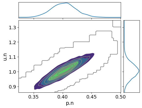
A third, more advanced method to perform uncertainty quantification is Bayesian statistics. Bayesian statistics is based on a different statistical foundation than Frequentist methods. The result of Bayesian statistics is a multivariate probability distribution (posterior) that encodes likely parameter combinations by placing probability mass on them. These probability distributions are numerically computed by non-uniform Markov Chain Monte Carlo sampling.

samples = x3cflux.run_non_uniform_sampling(simulator, num_samples=5_000, thinning=2, starting_point=np.array([.5, 1.4]),
                                           proposal=hopsy.CSmMALAProposal, progress_bar=True)

chain 0: 100%|██████████| 5000/5000 [00:02<00:00, 1729.65it/s]

The samples from the posterior distribution can e.g. be visualized and further analized by expert software packages like arviz

arviz.plot_pair(arviz.from_dict({simulator.parameter_space.free_parameter_names[i]: samples[:, i, :].flatten()
                                 for i in range(simulator.parameter_space.num_free_parameters)}),
                marginals=True, kind="kde")
plt.show()

Comparison of uncertainty estimates

we can now compare the uncertainty estiamtes for 95% confidence/credible interval

linearized_intervals = np.vstack([optimum - 2*np.sqrt(np.diag(cov)), optimum + 2*np.sqrt(np.diag(cov))])
plike_intervals = np.flip(np.reshape(pl_intervals[:2], (2,2)).transpose(),axis=1)
credible_intervals = np.quantile(samples[0],[0.025,0.975], axis=1)
print(optimum)
print(linearized_intervals)
print(plike_intervals)

[0.40001103 1.00002669]
[[0.35627867 0.90002669]
 [0.44374338 1.10002669]]
[[0.35782236 0.90236783]
 [0.44324823 1.09768229]]

variables = simulator.parameter_space.free_parameter_names
x = np.arange(len(variables))  # x locations for the groups
width = 0.2
fig, ax = plt.subplots()

ax.bar(x - width, linearized_intervals[1, :] - linearized_intervals[0, :], width,
       bottom=linearized_intervals[0, :], label='Linearized')
ax.bar(x, plike_intervals[1, :] - plike_intervals[0, :], width,
       bottom=plike_intervals[0, :], label='Profile likelihood')
ax.bar(x + width, credible_intervals[1, :] - credible_intervals[0, :], width,
       bottom=credible_intervals[0, :], label='Bayesian')

ax.set_xlabel('Variables')
ax.set_ylabel('Values')
plt.legend()
ax.set_xticks(x)
_ = ax.set_xticklabels(variables)

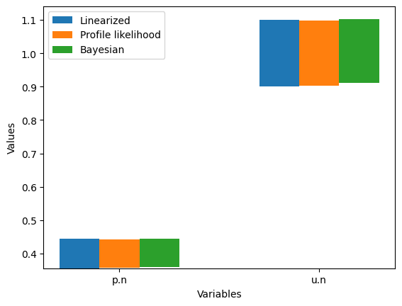
Which, in this simple case, are virtually identical. This was evident from the elliptical and highly symmetrical shape of the Bayesian posterior.

INST

13CFLUX can also handle isotopically non-stationary 13C-MFA through the same interface

simulator_inst = x3cflux.create_simulator_from_fml("spiralus.fml", "ms_INST")

Pool size of metabolite "G" is non-determinable given the measurement configuration, as it does not impact the simulation outcome. Consider fixing the pool size in FluxML to reduce the ill-conditionedness of the inverse problem.

The simulator informs us, that the pool size of G has no influence on the simulated measurements. We verify this by trying two different values for it.

param_names_inst = simulator_inst.parameter_space.free_parameter_names
params_inst = x3cflux.get_parameters(simulator_inst.parameter_space, simulator_inst.configurations[0].parameter_entries)
print("current parameter values")
for n, v in zip(param_names_inst, params_inst):
    print(f"{n}: {v}")

current parameter values
q.n: 0.6
u.n: 1.0
G: 1.0
B: 1.0
Pool size "G" not set in initial configuration (set to 1)

for p in [[0.6, 1, 0.2, 1],[0.6, 1, 1, 1], [0.6, 1, 5, 1]]:
    print(f"residual at {p}: {simulator_inst.compute_loss(p)}")

residual at [0.6, 1, 0.2, 1]: 0.00011629149758229874
residual at [0.6, 1, 1, 1]: 0.00011629149758229874
residual at [0.6, 1, 5, 1]: 0.00011629149758229874

simulator_inst.compute_loss([0.6, 1, 5, 1])

0.00011629149758229874

Indeed, the residual is identical regardless whether the pool size of G is 0.2, 1 or 5.

Hence, we fix it to 1 and also remove it from the parameters of the simulation.

config = simulator_inst.configurations[0]
pool_constr = config.pool_size_constraints
# Add constraint for G
def_constr = [constr for constr in pool_constr.definition_constraints] + [x3cflux.DefinitionConstraint(name="manual_constraint", parameter_name="G", parameter_value=1)]
# build new configuration
pool_constr = x3cflux.ParameterConstraints(def_constr, pool_constr.equality_constraints, pool_constr.inequality_constraints)
new_config = x3cflux.MeasurementConfiguration(
    config.name,
    config.comment,
    config.stationary,
    config.substrates,
    config.measurements,
    config.net_flux_constraints,
    config.exchange_flux_constraints,
    pool_constr,
    [x for x in simulator_inst.configurations[0].parameter_entries if x.name != 'G']) # remove G from parameters
simulator_inst = x3cflux.create_simulator_from_data(simulator_inst.network_data, new_config)

The simulator no longer indicates a non-determinable pool size and our parameters are now:

param_names_inst = simulator_inst.parameter_space.free_parameter_names
params_inst = x3cflux.get_parameters(simulator_inst.parameter_space, simulator_inst.configurations[0].parameter_entries)
for n, v in zip(param_names_inst, params_inst):
    print(f"{n}: {v}")

q.n: 0.6
u.n: 1.0
B: 1.0

Configuring the simulator

13CFLUX offers two different solvers for the differential equations (“bdf”, “sdirk”), and allows to set the relative and absolute solver tolerances.

simulator_inst.builder.set_solver("bdf")
simulator_inst.builder.solver.relative_tolerance = 1e-4
simulator_inst.builder.solver.absolute_tolerance = 1e-7
simulator_inst.builder.derivative_solver.relative_tolerance = 1e-4
simulator_inst.builder.derivative_solver.absolute_tolerance = 1e-7

Forward simulation

In case of INST, also the times at which the forward simulation is evaluated can be set.

First we define some common settings

offset = 0.2
times = np.geomspace(start=offset, stop=20+offset, num=50)-offset
meas_times = simulator_inst.measurement_time_stamps[0]
almost_infty = 1e5

Now for the actual simulation

ms=simulator_inst.compute_measurements(params=params_inst, time_stamps=times)[0]
ms_infty=simulator_inst.compute_measurements(params=params_inst, time_stamps=[almost_infty])[0][0]
ax = pd.DataFrame(np.vstack(ms),columns=["M+0", "M+1", "M+2"], index=times).plot()
ax.scatter([25,25,25],[ms_infty], marker='x', color=[
    ax.get_lines()[0].get_color(),
    ax.get_lines()[1].get_color(),
    ax.get_lines()[2].get_color()])
ax.set_ylim([0,1])
ax.set_xticks(np.arange(0,26,5))
_ = ax.set_xticklabels([0,5,10,15,20, "∞"])
for t in meas_times:
    ax.plot([t,t], [0,1], 'k--')
ax.set_xlim([0,26])

(0.0, 26.0)

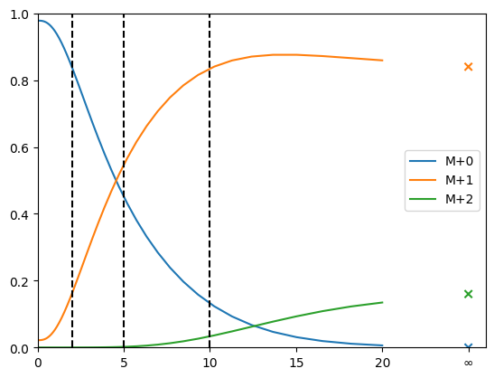
The colored lines show the timecourse of the labeling, dashed lines indicate time points of measurements. the x-es at ∞ show the stationary solution.

If we now increase the pool size of B (the first pool after the input), the labeling dynamics is significantly slowed down

params_inst2 = params_inst.copy()
params_inst2[2] = 10 # set B to 10
ms=simulator_inst.compute_measurements(params=params_inst2, time_stamps=times)[0]
ms_infty=simulator_inst.compute_measurements(params=params_inst2, time_stamps=[almost_infty])[0][0]
ax = pd.DataFrame(np.vstack(ms),columns=["M+0", "M+1", "M+2"], index=times).plot()
ax.scatter([25,25,25],[ms_infty], marker='x', color=[
    ax.get_lines()[0].get_color(),
    ax.get_lines()[1].get_color(),
    ax.get_lines()[2].get_color()])
ax.set_ylim([0,1])
ax.set_xticks(np.arange(0,26,5))
_ = ax.set_xticklabels([0,5,10,15,20, "∞"])
for t in meas_times:
    ax.plot([t,t], [0,1], 'k--')
_ = ax.set_xlim([0,26])

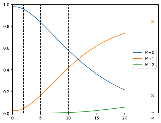
The stationary solution, as expected, is not affected by the change in pool size.

Optimization + Statistics

Optimization and statistics work exactly the same as for the stationary case:

• Fitting

optimum_inst, obj_val = x3cflux.run_optimization(simulator_inst,
                                            starting_point=np.array([0.5, 1.2, 0.5]),
                                            max_iter=100,
                                            tol=1e-3)
print(f"Optimum at {optimum_inst} with and objective value of {obj_val}")

Optimum at [0.6002588  1.00019754 1.00134517] with and objective value of 6.429128063154018e-05

• Linearized statistics

cov_inst, non_ident = x3cflux.compute_free_parameter_covariance(simulator_inst, optimum_inst)
print(f"Covariance Matrix at {optimum}:\n {cov_inst}")
print(f"List of non-identifiable parameters: {non_ident}")

Covariance Matrix at [0.40001103 1.00002669]:
 [[0.00116501 0.00090038 0.00707814]
 [0.00090038 0.00115914 0.00603928]
 [0.00707814 0.00603928 0.04600468]]
List of non-identifiable parameters: []

• Profile likelihood

alpha=0.95
names=["q.n", "u.n", "B"]
pl_intervals_inst = x3cflux.run_profile_likelihood_cis(simulator_inst, optimum_inst, alpha=alpha, names=names, num_procs=4)
print(f"{100*alpha}% confidence intervals")
for n,i in zip(names, pl_intervals_inst):
    print(f"{i[0]} < {n} < {i[1]}")

95.0% confidence intervals
0.5448638261590698 < q.n < 0.6824317044057978
0.9406154569582612 < u.n < 1.0753891358262595
0.6533094368930802 < B < 1.5170761781099686

• Bayesian statistics

samples_inst = x3cflux.run_non_uniform_sampling(simulator_inst, num_samples=5_000, thinning=3, starting_point=np.array([.3, 1.1, 0.9]),
                                           proposal=hopsy.CSmMALAProposal, progress_bar=True)

chain 0: 100%|██████████| 5000/5000 [02:09<00:00, 38.74it/s]

arviz.plot_pair(arviz.from_dict({simulator_inst.parameter_space.free_parameter_names[i]: samples_inst[:, i, :].flatten()
                                 for i in range(simulator_inst.parameter_space.num_free_parameters)}),
                marginals=True, kind="kde")
plt.show()

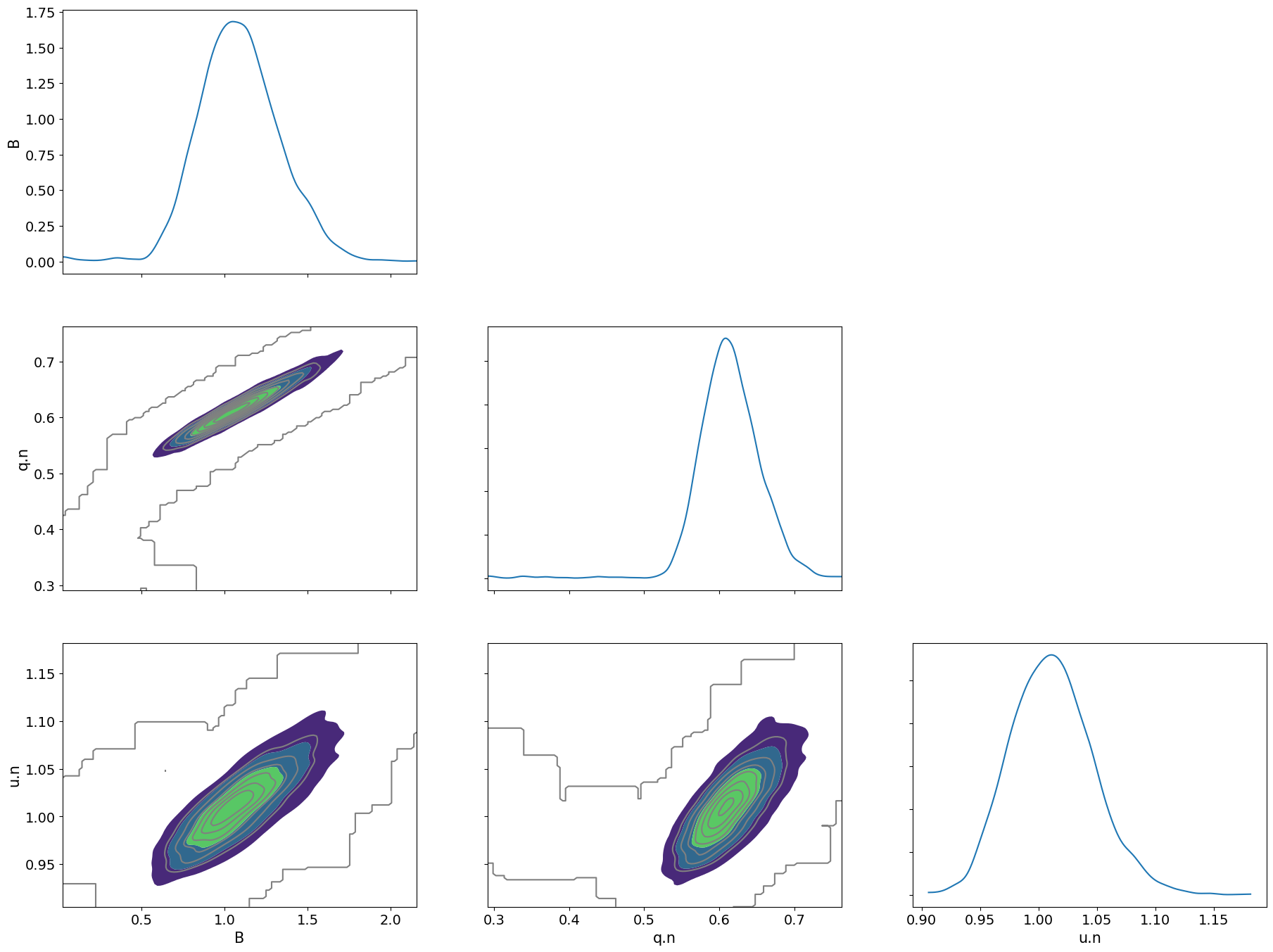
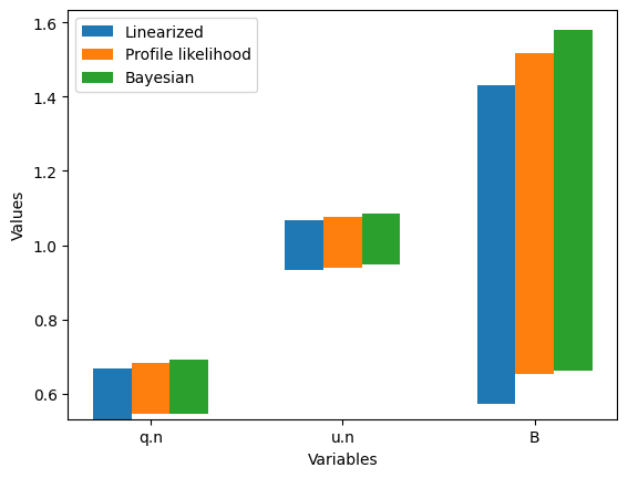
Finally, we can compare them again:

linearized_intervals_inst = np.vstack([optimum_inst - 2*np.sqrt(np.diag(cov_inst)), optimum_inst + 2*np.sqrt(np.diag(cov_inst))])
plike_intervals_inst = np.transpose(pl_intervals_inst)
credible_intervals_inst = np.quantile(samples_inst[0],[0.025,0.975], axis=1)

variables_inst = simulator_inst.parameter_space.free_parameter_names
x = np.arange(len(variables_inst))  # x locations for the groups
width = 0.2
fig, ax = plt.subplots()

ax.bar(x - width, linearized_intervals_inst[1, :] - linearized_intervals_inst[0, :], width,
       bottom=linearized_intervals_inst[0, :], label='Linearized')
ax.bar(x, plike_intervals_inst[1, :] - plike_intervals_inst[0, :], width,
       bottom=plike_intervals_inst[0, :], label='Profile likelihood')
ax.bar(x + width, credible_intervals_inst[1, :] - credible_intervals_inst[0, :], width,
       bottom=credible_intervals_inst[0, :], label='Bayesian')

ax.set_xlabel('Variables')
ax.set_ylabel('Values')
plt.legend()
ax.set_xticks(x)
_= ax.set_xticklabels(variables_inst)